getOutput
Arguments
- ConcreteEst
"ConcreteEst" object
- Estimand
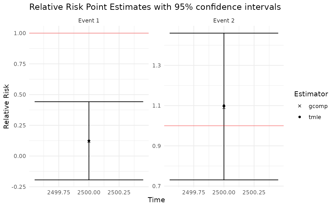
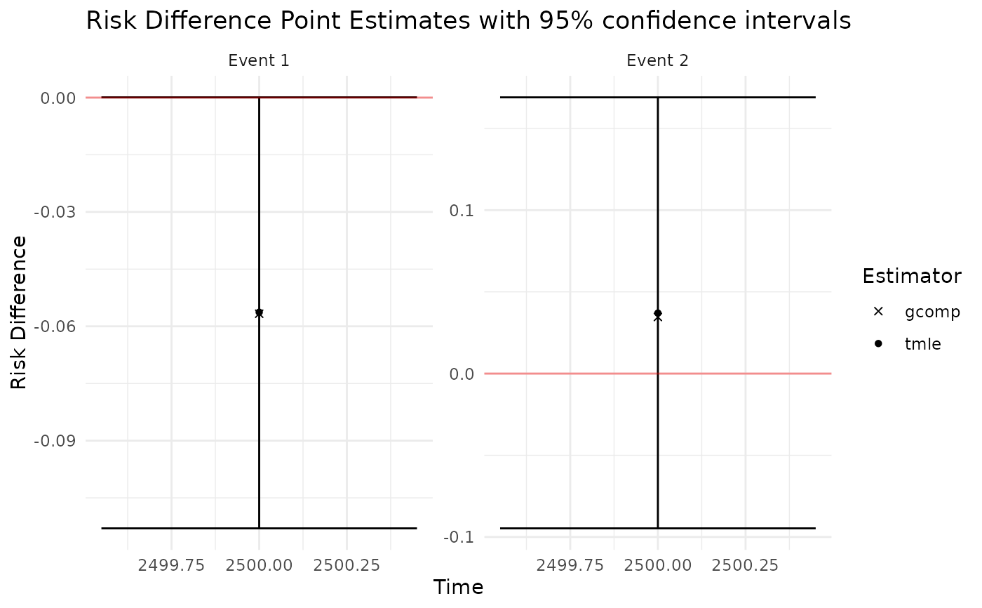
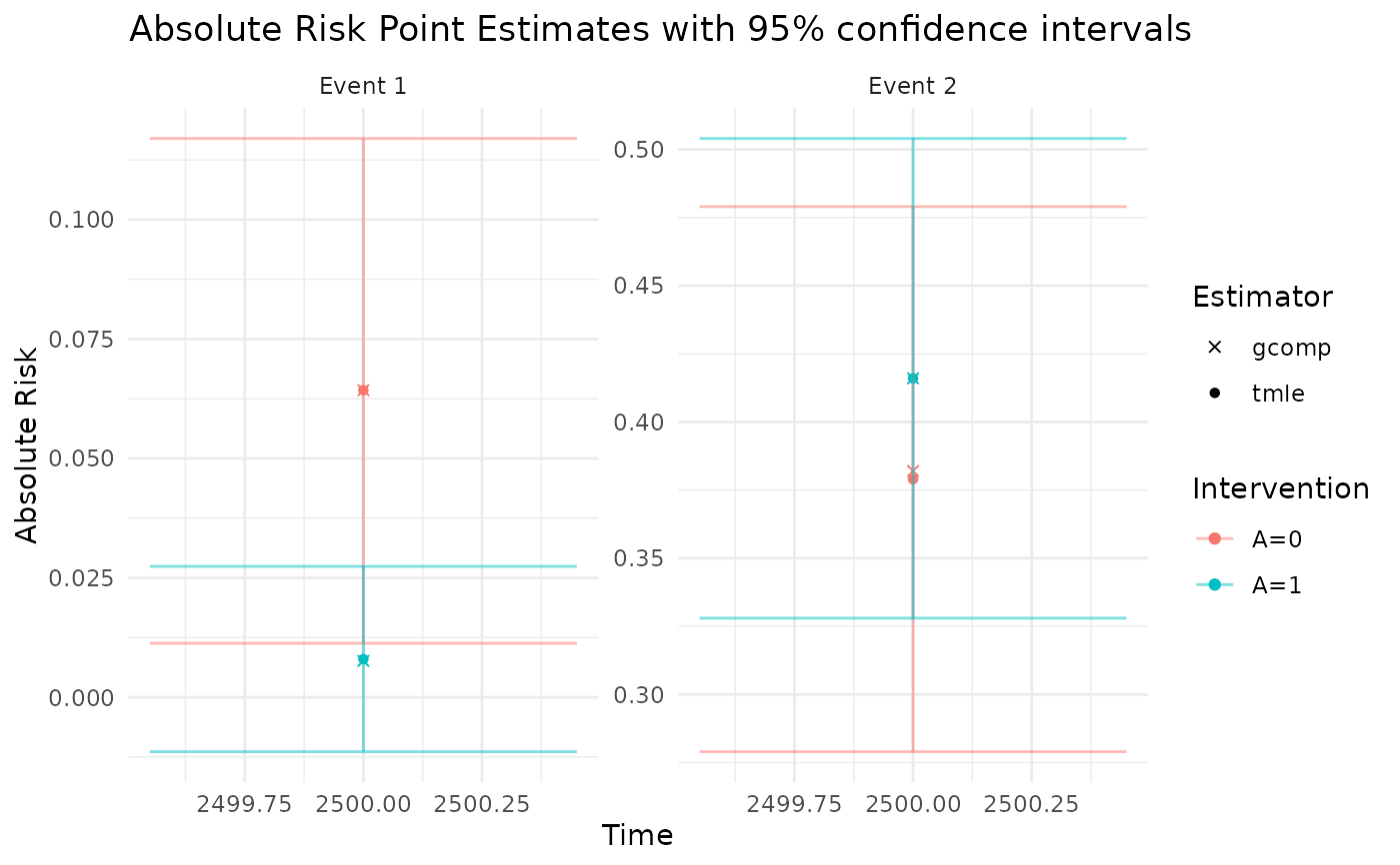
character: "RR" for Relative Risks, "RD" for Risk Differences, and "Risk" for absolute risks
- Intervention
numeric (default = seq_along(ConcreteEst)): the ConcreteEst list element corresponding to the target intervention. For comparison estimands such as RD and RR, Intervention should be a numeric vector with length 2, the first term designating "treatment" ConcreteEst list element and the second designating the "control".
- GComp
logical: return g-formula point estimates based on initial nuisance parameter estimation
- Simultaneous
logical: return simultaneous confidence intervals
- Signif
numeric (default = 0.05): alpha for 2-tailed hypothesis testing
- NIMargin
numeric (optional): a non-inferiority margin for the comparative (RD/RR) estimands. When supplied, a one-sided non-inferiority assessment is added (
NIpValue,NonInferior).- NIDirection
one of
"lower"or"upper": which side of the margin is "non-inferior". Use"upper"when a smaller estimate is better (the usual risk-difference case) and"lower"when larger is better.- x
a ConcreteOut object
- NullLine
logical: to plot a red line at y=1 for RR plots and at y=0 for RD plots
- ask
logical: to prompt for user input before each plot
- ...
additional arguments to be passed into plot methods
Value
data.table of point estimates and standard deviations. Comparative
estimands carry a two-sided Wald pValue. If the fit was built with
Strata (see formatArguments()), all standard errors are corrected for
the stratified / covariate-adaptive randomization design.
Examples
library(data.table)
library(concrete)

data <- as.data.table(survival::pbc)
data <- data[1:200, .SD, .SDcols = c("id", "time", "status", "trt", "age", "sex")]
data[, trt := sample(0:1, nrow(data), TRUE)]
#>         id  time status   trt      age    sex
#>      <int> <int>  <int> <int>    <num> <fctr>
#>   1:     1   400      2     1 58.76523      f
#>   2:     2  4500      0     1 56.44627      f
#>   3:     3  1012      2     1 70.07255      m
#>   4:     4  1925      2     1 54.74059      f
#>   5:     5  1504      1     0 38.10541      f
#>  ---
#> 196:   196  2363      0     0 57.04038      f
#> 197:   197  2365      0     0 44.62697      f
#> 198:   198  2357      0     0 35.79740      f
#> 199:   199  1592      0     0 40.71732      f
#> 200:   200  2318      0     1 32.23272      f

# formatArguments() returns correctly formatted arguments for doConcrete()
concrete.args <- formatArguments(DataTable = data,
                                 EventTime = "time",
                                 EventType = "status",
                                 Treatment = "trt",
                                 ID = "id",
                                 TargetTime = 2500,
                                 TargetEvent = c(1, 2),
                                 Intervention = makeITT(),
                                 CVArg = list(V = 2))

# doConcrete() returns tmle (and g-formula plug-in) estimates of targeted risks
# \donttest{
concrete.est <- doConcrete(concrete.args)
#>
#> Estimating Treatment Propensity:
#>
#> Estimating Hazards:
#> Warning: Loglik converged before variable  1 ; coefficient may be infinite.
#> Warning: Loglik converged before variable  1,3 ; coefficient may be infinite.
#>       Trt  Time Event         PnEIC RelativeCriteria     AbsPnEIC
#>    <char> <num> <num>         <num>            <num>        <num>
#> 1:    A=1  2500     1  0.0024001043      0.001867462 0.0024001043
#> 2:    A=0  2500     2 -0.0063702933      0.009615051 0.0063702933
#> 3:    A=1  2500     2 -0.0003148435      0.008512401 0.0003148435
#>    AbsoluteCriteria StopCriteria RelativeRatio AbsoluteRatio ratio StopRule
#>               <num>        <num>         <num>         <num> <num>   <char>
#> 1:                0  0.001867462    1.28522234           Inf  1.29 relative
#> 2:                0  0.009615051    0.66253349           Inf  0.66 relative
#> 3:                0  0.008512401    0.03698645           Inf  0.04 relative
#>    StopAbsTol
#>         <num>
#> 1:          0
#> 2:          0
#> 3:          0
#> Norm PnEIC = 0.006815149
#>
#> Starting TMLE Update:
#> Problem dimension: k = 4
#> Using standard universal LFM approach (iterative small steps)
#> Starting step 1 with update epsilon = 0.1
#> Update increased the active convergence objective, halving OneStepEps
#> Starting step 1 with update epsilon = 0.05
#> Update increased the active convergence objective, halving OneStepEps
#> Starting step 1 with update epsilon = 0.025
#>       Trt  Time Event        PnEIC RelativeCriteria    AbsPnEIC
#>    <char> <num> <num>        <num>            <num>       <num>
#> 1:    A=1  2500     1  0.002273792      0.001867383 0.002273792
#> 2:    A=0  2500     2  0.005521087      0.009612210 0.005521087
#> 3:    A=0  2500     1 -0.001209543      0.005107295 0.001209543
#>    AbsoluteCriteria StopCriteria RelativeRatio AbsoluteRatio ratio StopRule
#>               <num>        <num>         <num>         <num> <num>   <char>
#> 1:                0  0.001867383     1.2176357           Inf  1.22 relative
#> 2:                0  0.009612210     0.5743827           Inf  0.57 relative
#> 3:                0  0.005107295     0.2368266           Inf  0.24 relative
#>    StopAbsTol
#>         <num>
#> 1:          0
#> 2:          0
#> 3:          0
#> Norm PnEIC = 0.00609487
#> Starting step 2 with update epsilon = 0.025
#> Update increased the active convergence objective, halving OneStepEps
#> Starting step 2 with update epsilon = 0.0125
#>       Trt  Time Event         PnEIC RelativeCriteria     AbsPnEIC
#>    <char> <num> <num>         <num>            <num>        <num>
#> 1:    A=1  2500     1  0.0022111210      0.001867343 0.0022111210
#> 2:    A=0  2500     1 -0.0002390974      0.005107428 0.0002390974
#> 3:    A=0  2500     2 -0.0003917493      0.009613071 0.0003917493
#>    AbsoluteCriteria StopCriteria RelativeRatio AbsoluteRatio ratio StopRule
#>               <num>        <num>         <num>         <num> <num>   <char>
#> 1:                0  0.001867343    1.18410037           Inf  1.18 relative
#> 2:                0  0.005107428    0.04681366           Inf  0.05 relative
#> 3:                0  0.009613071    0.04075173           Inf  0.04 relative
#>    StopAbsTol
#>         <num>
#> 1:          0
#> 2:          0
#> 3:          0
#> Norm PnEIC = 0.002259054
#> Starting step 3 with update epsilon = 0.0125
#>       Trt  Time Event         PnEIC RelativeCriteria     AbsPnEIC
#>    <char> <num> <num>         <num>            <num>        <num>
#> 1:    A=1  2500     1  0.0020409249      0.001867236 0.0020409249
#> 2:    A=0  2500     2  0.0006443768      0.009612840 0.0006443768
#> 3:    A=0  2500     1 -0.0001587924      0.005107558 0.0001587924
#>    AbsoluteCriteria StopCriteria RelativeRatio AbsoluteRatio ratio StopRule
#>               <num>        <num>         <num>         <num> <num>   <char>
#> 1:                0  0.001867236    1.09301931           Inf  1.09 relative
#> 2:                0  0.009612840    0.06703293           Inf  0.07 relative
#> 3:                0  0.005107558    0.03108968           Inf  0.03 relative
#>    StopAbsTol
#>         <num>
#> 1:          0
#> 2:          0
#> 3:          0
#> Norm PnEIC = 0.002146123
#> Starting step 4 with update epsilon = 0.0125
#> Update increased the active convergence objective, halving OneStepEps
#> Starting step 4 with update epsilon = 0.00625
#>       Trt  Time Event         PnEIC RelativeCriteria     AbsPnEIC
#>    <char> <num> <num>         <num>            <num>        <num>
#> 1:    A=1  2500     1  1.955942e-03      0.001867184 1.955942e-03
#> 2:    A=0  2500     2 -3.386572e-04      0.009613055 3.386572e-04
#> 3:    A=1  2500     2  3.232335e-05      0.008512313 3.232335e-05
#>    AbsoluteCriteria StopCriteria RelativeRatio AbsoluteRatio ratio StopRule
#>               <num>        <num>         <num>         <num> <num>   <char>
#> 1:                0  0.001867184   1.047535643           Inf  1.05 relative
#> 2:                0  0.009613055   0.035228883           Inf  0.04 relative
#> 3:                0  0.008512313   0.003797247           Inf  0.00 relative
#>    StopAbsTol
#>         <num>
#> 1:          0
#> 2:          0
#> 3:          0
#> Norm PnEIC = 0.001985325
#> Starting step 5 with update epsilon = 0.00625
#>       Trt  Time Event         PnEIC RelativeCriteria     AbsPnEIC
#>    <char> <num> <num>         <num>            <num>        <num>
#> 1:    A=1  2500     1  1.867586e-03      0.001867131 1.867586e-03
#> 2:    A=0  2500     2  2.071158e-04      0.009612931 2.071158e-04
#> 3:    A=0  2500     1 -5.176869e-05      0.005107594 5.176869e-05
#>    AbsoluteCriteria StopCriteria RelativeRatio AbsoluteRatio ratio StopRule
#>               <num>        <num>         <num>         <num> <num>   <char>
#> 1:                0  0.001867131    1.00024373           Inf  1.00 relative
#> 2:                0  0.009612931    0.02154554           Inf  0.02 relative
#> 3:                0  0.005107594    0.01013563           Inf  0.01 relative
#>    StopAbsTol
#>         <num>
#> 1:          0
#> 2:          0
#> 3:          0
#> Norm PnEIC = 0.001879926
#> Starting step 6 with update epsilon = 0.00625
#>       Trt  Time Event         PnEIC RelativeCriteria     AbsPnEIC
#>    <char> <num> <num>         <num>            <num>        <num>
#> 1:    A=1  2500     1  1.777413e-03      0.001867078 1.777413e-03
#> 2:    A=0  2500     2 -1.536649e-04      0.009613012 1.536649e-04
#> 3:    A=1  2500     2  2.615163e-05      0.008512319 2.615163e-05
#>    AbsoluteCriteria StopCriteria RelativeRatio AbsoluteRatio ratio StopRule
#>               <num>        <num>         <num>         <num> <num>   <char>
#> 1:                0  0.001867078   0.951975869           Inf  0.95 relative
#> 2:                0  0.009613012   0.015985094           Inf  0.02 relative
#> 3:                0  0.008512319   0.003072211           Inf  0.00 relative
#>    StopAbsTol
#>         <num>
#> 1:          0
#> 2:          0
#> 3:          0
#> Norm PnEIC = 0.001784263

# getOutput returns risk difference, relative risk, and treatment-specific risks
#  GComp=TRUE returns g-formula plug-in estimates
#  Simultaneous=TRUE computes simultaneous CI for all output TMLE estimates
concrete.out <- getOutput(concrete.est, Estimand = c("RR", "RD", "Risk"),
                          GComp = TRUE, Simultaneous = TRUE)
print(concrete.out)
#>      Time Event  Estimand  Intervention Estimator   Pt Est      se  CI Low
#>     <num> <num>    <char>        <char>    <char>    <num>   <num>   <num>
#>  1:  2500     1  Abs Risk           A=0      tmle  0.06430 0.02710  0.0113
#>  2:  2500     1  Abs Risk           A=0     gcomp  0.06430      NA      NA
#>  3:  2500     1  Abs Risk           A=1      tmle  0.00798 0.00989 -0.0114
#>  4:  2500     1  Abs Risk           A=1     gcomp  0.00762      NA      NA
#>  5:  2500     1  Rel Risk [A=1] / [A=0]      tmle  0.12400 0.16200 -0.1940
#>  6:  2500     1  Rel Risk [A=1] / [A=0]     gcomp  0.11800      NA      NA
#>  7:  2500     1 Risk Diff [A=1] - [A=0]      tmle -0.05630 0.02880 -0.1130
#>  8:  2500     1 Risk Diff [A=1] - [A=0]     gcomp -0.05670      NA      NA
#>  9:  2500     2  Abs Risk           A=0      tmle  0.37900 0.05090  0.2790
#> 10:  2500     2  Abs Risk           A=0     gcomp  0.38200      NA      NA
#> 11:  2500     2  Abs Risk           A=1      tmle  0.41600 0.04510  0.3280
#> 12:  2500     2  Abs Risk           A=1     gcomp  0.41600      NA      NA
#> 13:  2500     2  Rel Risk [A=1] / [A=0]      tmle  1.10000 0.18700  0.7310
#> 14:  2500     2  Rel Risk [A=1] / [A=0]     gcomp  1.09000      NA      NA
#> 15:  2500     2 Risk Diff [A=1] - [A=0]      tmle  0.03700 0.06720 -0.0947
#> 16:  2500     2 Risk Diff [A=1] - [A=0]     gcomp  0.03460      NA      NA
#>        CI Hi SimCI Low SimCI Hi  pValue
#>        <num>     <num>    <num>   <num>
#>  1: 1.17e-01  -0.00459   0.1330      NA
#>  2:       NA        NA       NA      NA
#>  3: 2.74e-02  -0.01720   0.0332      NA
#>  4:       NA        NA       NA      NA
#>  5: 4.42e-01  -0.28900   0.5370 6.7e-08
#>  6:       NA        NA       NA      NA
#>  7: 6.33e-05  -0.13000   0.0169 5.0e-02
#>  8:       NA        NA       NA      NA
#>  9: 4.79e-01   0.24900   0.5090      NA
#> 10:       NA        NA       NA      NA
#> 11: 5.04e-01   0.30100   0.5310      NA
#> 12:       NA        NA       NA      NA
#> 13: 1.46e+00   0.62100   1.5700 6.0e-01
#> 14:       NA        NA       NA      NA
#> 15: 1.69e-01  -0.13400   0.2080 5.8e-01
#> 16:       NA        NA       NA      NA
plot(concrete.out, ask = FALSE)


# }
# }