How concrete works

This article explains what concrete computes and how the algorithm gets there. It is written for analysts who want intuition for the estimator behind the trial outputs, without reading the full methods paper. The schematic figures below are teaching illustrations of the algorithm, not simulation results; see the Simulation evidence article for empirical bias and coverage.

The method is one-step continuous-time targeted minimum loss-based estimation (TMLE) for cause-specific absolute risks, following Rytgaard et al. (2023) and Rytgaard and van der Laan (2023).

The target: a covariate-adjusted absolute risk

For a binary baseline treatment a and baseline covariates W, the conditional cause-j absolute risk by time t is the cumulative incidence

$$F_j(t \mid a, W) = \int_0^t \lambda_j(s \mid a, W)\, S(s^- \mid a, W)\, ds, \qquad S(t \mid a, W) = \exp\!\Big(\!-\!\int_0^t \textstyle\sum_{j=1}^J \lambda_j(s\mid a,W)\, ds\Big),$$

where $\lambda_j$ is the cause-j hazard and $S$ is the overall event-free survival across all $J$ competing events. The trial estimand is the marginal risk under an intervention, averaged over the covariate distribution:

$$\Psi_{j,t} = \mathbb{E}_W\big[\, F_j(t \mid a, W)\, \big],$$

and from a pair of interventions concrete reports the risk difference and risk ratio. Censoring is treated as a competing event (0) and handled through inverse-probability-of-censoring weighting inside the estimator, not by discarding censored subjects.

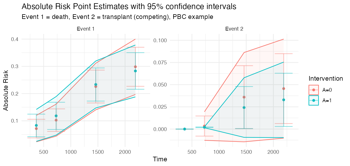
With competing risks, each event gets its own cause-specific cumulative incidence. The figure below is real concrete output on the PBC example, with death (event 1) and transplant (event 2, the competing event) targeted jointly:

The pipeline

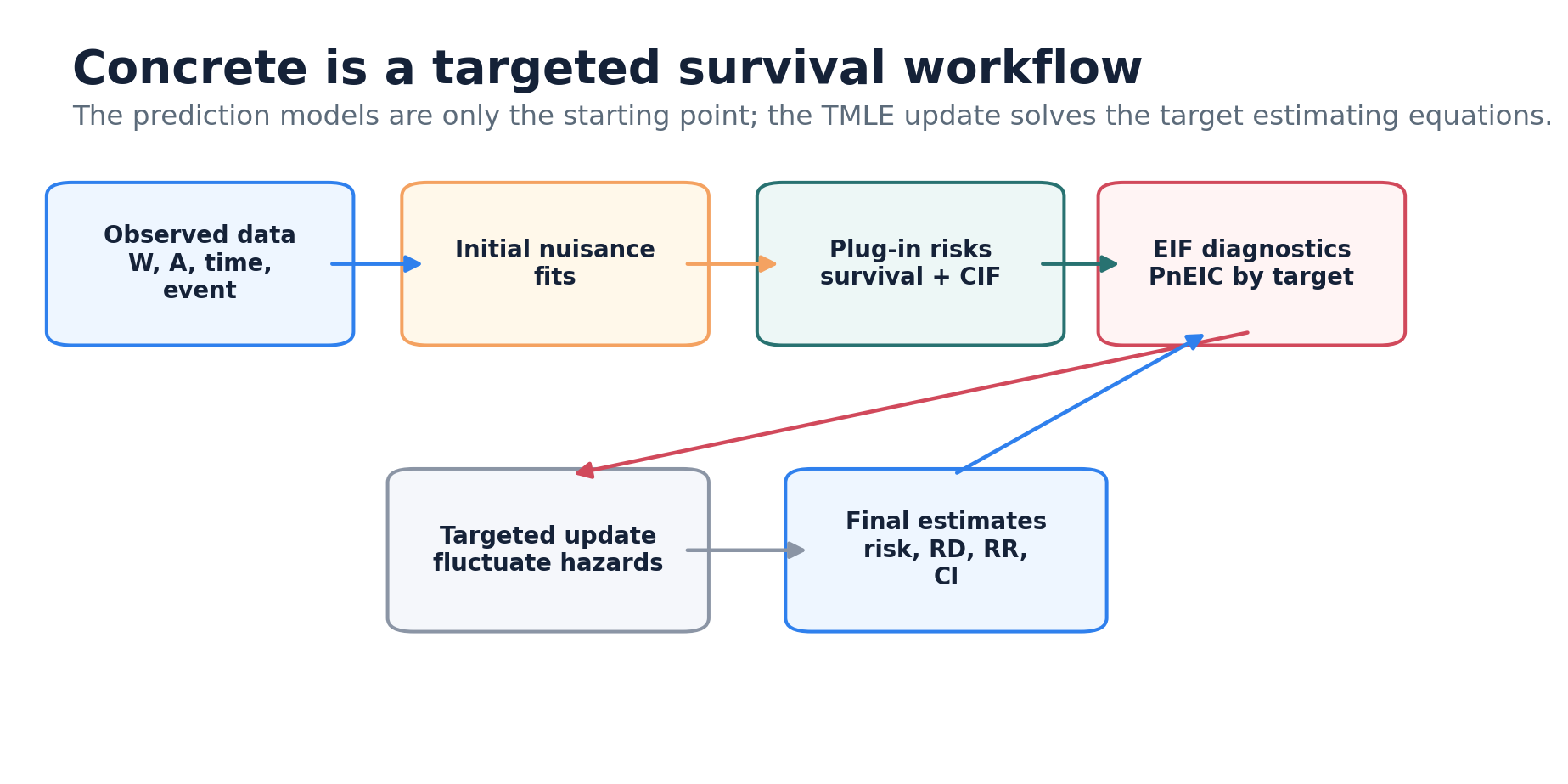
concrete runs four stages:

1. Estimate nuisance parameters. A treatment Super Learner estimates the propensity score pi(a | W); event-specific and censoring hazard libraries (Cox, Coxnet, random survival forests, additive hazards, HAL) are fit with cross-validated selection.
2. Form the initial plug-in. The hazards are turned into per-subject cumulative-incidence curves and averaged to a first estimate of each risk.
3. Target. A small multiplicative update is applied to the hazards, repeatedly, to solve the efficient-influence-function (EIF) estimating equation for the requested risks.
4. Report. Point estimates, influence-function standard errors, and pointwise plus simultaneous confidence intervals for risks, differences, and ratios.

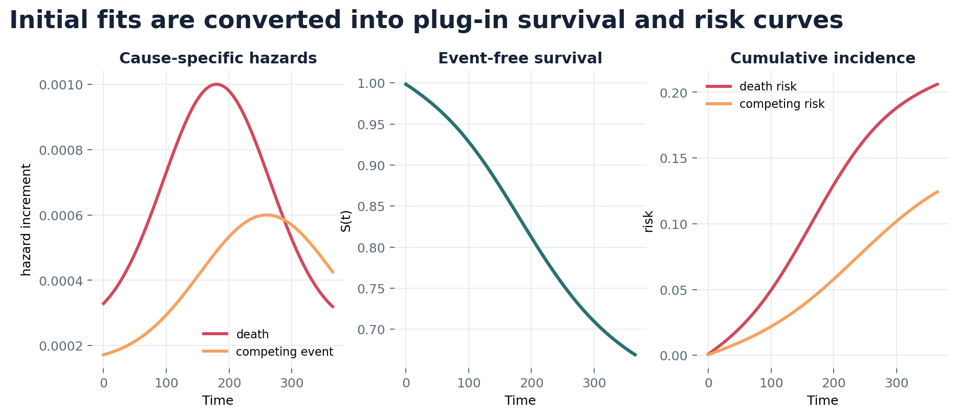
Step 1-2: an event-time grid and an initial plug-in

Continuous-time hazards are evaluated on the grid of observed event/censoring times together with the requested target times.

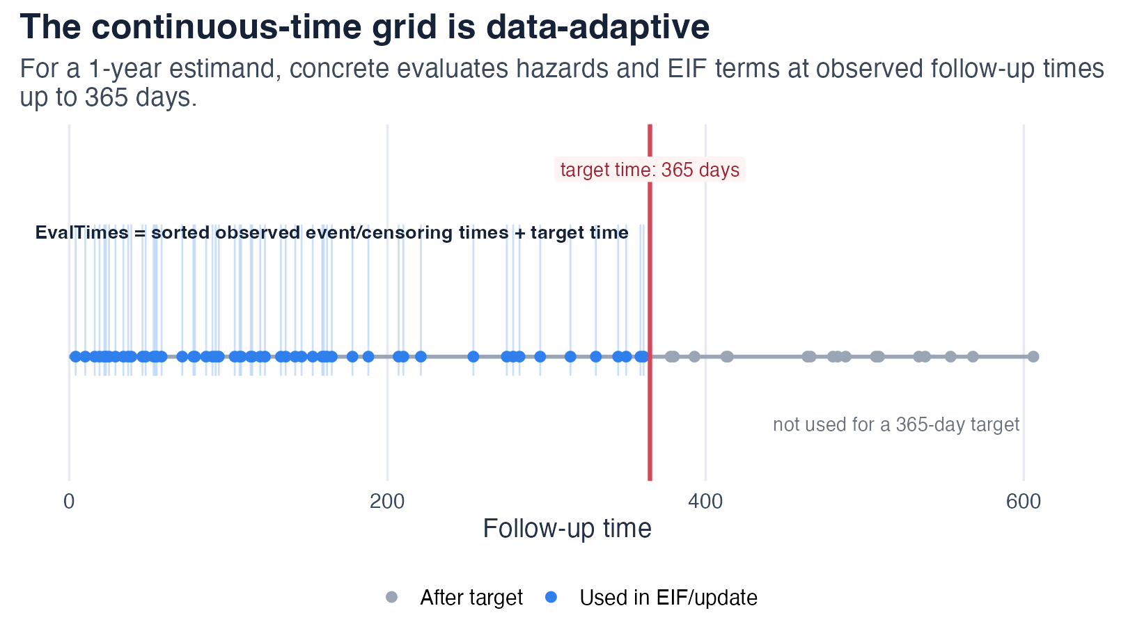
Cumulating the hazards along this grid gives each subject’s plug-in cumulative-incidence curve; averaging over subjects gives the initial risk estimate. This plug-in is consistent only if the hazard models are correct, and it is generally biased for the marginal risk because the learners optimize hazard fit rather than the target.

Step 3: the efficient influence function

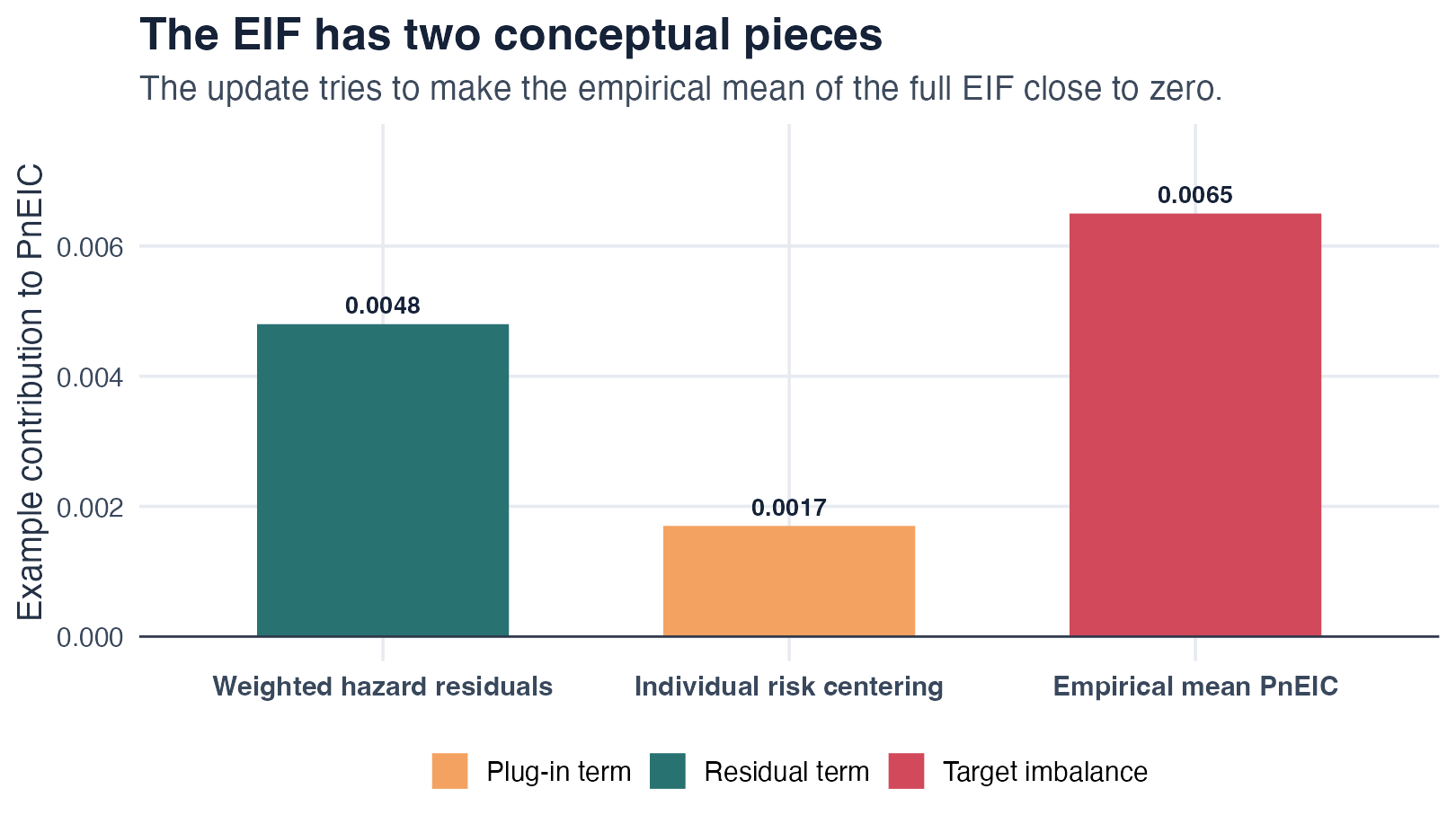
TMLE removes the plug-in bias by solving the EIF estimating equation. For target event j and time t, the EIF of each subject has three conceptual pieces:

$$D^*_{j,t}(O) \;=\; \underbrace{\sum_{l=1}^{J} \int_0^{t} h_{l,j,t}(s)\,\big(dN_l(s) - \mathbf{1}(\widetilde T \ge s)\,\lambda_l(s\mid A,W)\,ds\big)}_{\text{weighted hazard residuals}} \;+\; \underbrace{F_j(t \mid A, W) - \Psi_{j,t}}_{\text{individual risk centering}} .$$

The clever covariate $h$ weights each cause-l hazard residual by how much that hazard, at time s, moves the cause-j risk at time t:

$$h_{l,j,t}(s) \;=\; \frac{\pi^*(A\mid W)\,\mathbf{1}(s \le t)}{\pi(A\mid W)\, S_c(s^-\mid A, W)} \left(\mathbf{1}(l=j) - \frac{F_j(t\mid A,W) - F_j(s\mid A,W)}{S(s\mid A,W)}\right).$$

The first factor is the treatment/censoring weight — the intervention propensity $\pi^*$ over the observed propensity $\pi$ and the lagged probability of remaining uncensored $S_c(s^-)$. The MinNuisance bound is applied to this denominator to keep the weight stable under near-positivity violations. The empirical mean of the EIF over subjects, PnEIC, measures how far the current estimate is from solving the estimating equation; the update drives it toward zero.

Step 3: the targeting loop

concrete does not re-fit the hazards. It applies a single multiplicative fluctuation to every cause-l hazard, in the direction that most reduces the PnEIC, with a small step size $\varepsilon$:

$$\lambda_l^{b+1}(s) \;=\; \lambda_l^{b}(s)\, \exp\!\Big(\varepsilon\,\tfrac{\langle \mathbb{P}_n D^*,\, h_{l,\cdot}\rangle}{\lVert \mathbb{P}_n D^*\rVert}\Big).$$

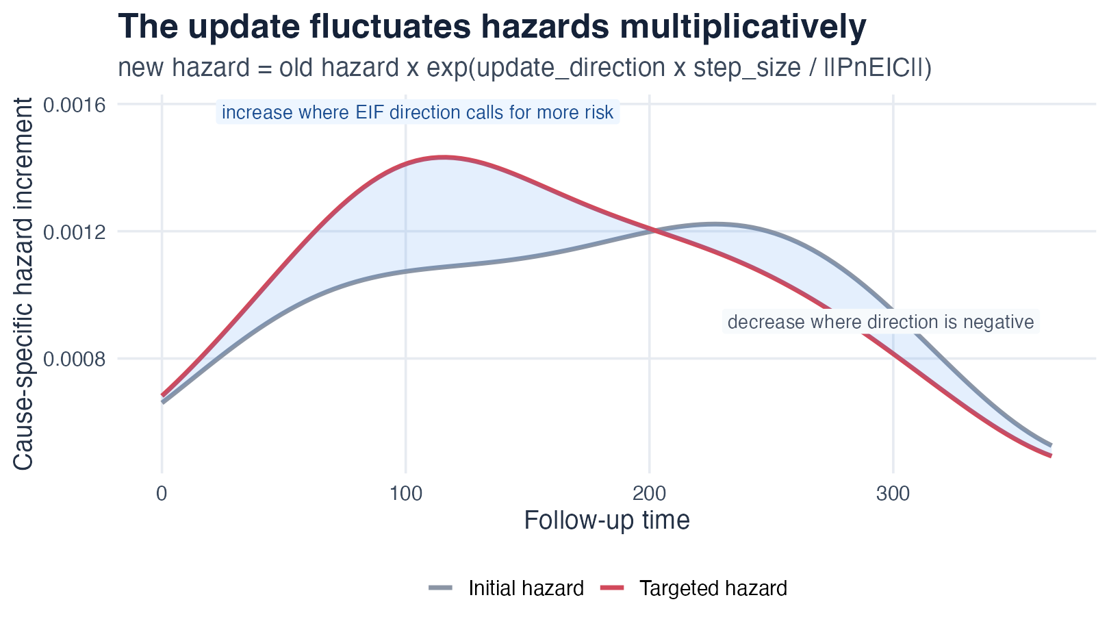
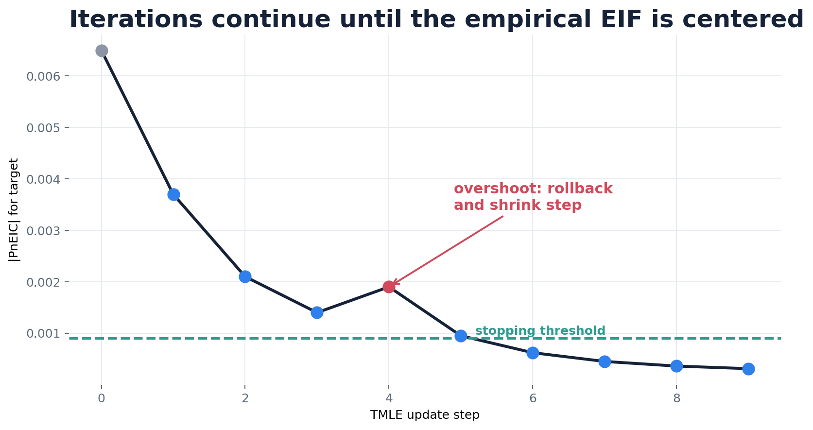
After each step the survival, cumulative incidence, and EIF are recomputed and the norm of the PnEIC is checked. The "adaptive" update method backtracks the step size whenever a step would increase the objective, so the norm decreases monotonically.

Direct targeting of derived functionals

The loop above targets the absolute risks at the chosen target times. Estimands derived from the risk curves — the RMST (a time-integral) and the win ratio (a bilinear functional of the two arms’ curves) — can be computed by plugging in those targeted curves, but the plug-in inherits the target-time grid (a trapezoid or Riemann sum over a few points) and never solves the derived functional’s own estimating equation.

targetRMST() and targetWinRatio() instead run the same fluctuation machinery with the derived functional’s clever covariate: by the chain rule, it is the gradient-weighted combination of the pointwise clever covariates over the full event-time grid — integral weights $(\tau - s)$ for the RMST, the win-functional’s exact discrete gradients for the win ratio (which depend on both arms’ current curves, so they are recomputed each step and both arms fluctuate jointly). The loop stops when the functional’s own $\mathbb{P}_n D^*$ is solved. In simulation this removes the grid sensitivity and cuts the residual bias several-fold for both estimands; see the RMST methods comparison and the win ratio articles for the numbers.

Step 3: when to stop

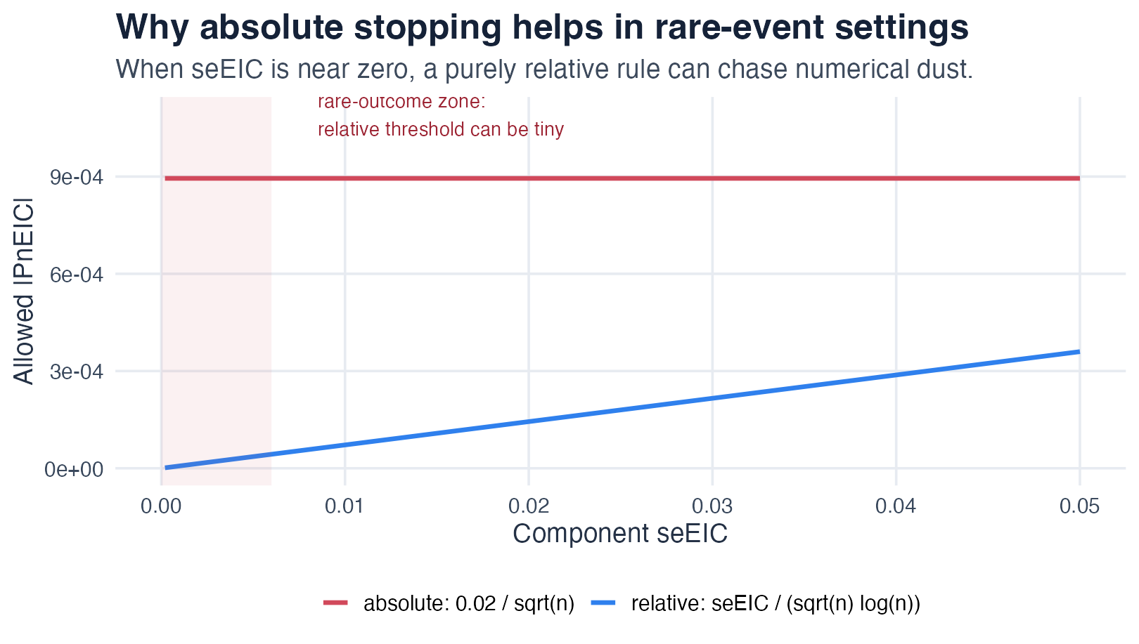
The loop stops when every targeted component has a small enough PnEIC. The relative rule compares |PnEIC| to its own standard-error scale, seEIC / (sqrt(n) * log(n)). In rare-event or competing-risk targets this threshold can become numerically tiny, so an absolute rule (|PnEIC| <= EICStopAbsTol, default 0.02 / sqrt(n)) is often more stable; the hybrid rule takes the larger of the two.

getTmleDiagnostics() reports, per component, the PnEIC, the active StopCriteria, their ratio, and whether the check passed. The Convergence diagnostics article shows how to read these and what to change when a fit does not converge cleanly.

Step 4: inference

The estimated EIF is also the basis for inference. The standard error of each risk is the influence-function standard deviation over sqrt(n). Risk differences and risk ratios use the paired per-subject influence functions of the two interventions (a delta-method transform for the ratio), so the correlation between arms is accounted for. With more than one target time, getOutput(Simultaneous = TRUE) adds simultaneous confidence bands using a multiplier-bootstrap maximum over the correlated component influence functions.

The iid influence-function variance assumes simple randomization. When the trial randomized within strata using a strong-balance scheme (permuted blocks, stratified biased coin), that variance is conservative: the design removes the between-arm-within-stratum component $\pi(1-\pi)\sum_s p_s \Delta(s)^2$, where $\Delta(s)$ is the between-arm difference of within-stratum means of the influence function. Passing the stratum columns as Strata to formatArguments() subtracts exactly that component (computed in a nonnegative residual-plus-between-stratum form) from the variance of every reported estimand — risks, RD/RR, RMST, and the win ratio. When the working models adjust for the stratification variables, $\Delta(s) \approx 0$ and the correction vanishes; see the regulatory toolkit for usage and caveats.

Where to go next

• Trialist quickstart: run it on your data.
• Learner library: choose nuisance learners.
• Convergence diagnostics: read and fix the stopping diagnostics.
• Simulation evidence: empirical bias and coverage.