Convergence diagnostics

This article explains how to evaluate the TMLE update when concrete reports slow convergence or non-convergence. The goal is to distinguish a meaningful targeting problem from a numerically tiny empirical efficient influence curve (EIC) component in a rare-event setting.

The illustrative code snippets assume a trial data.table and a fitted ConcreteEst object as built in the Trialist quickstart.

What convergence means here

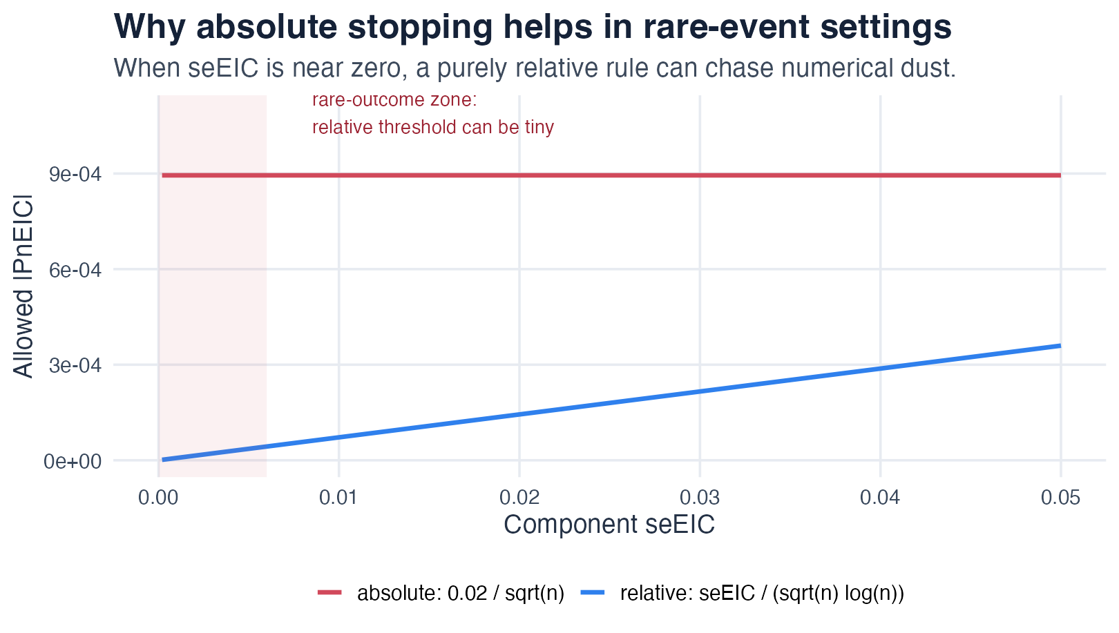
The TMLE update tries to make the empirical mean of each requested target EIC component small. Stopping is evaluated for the requested intervention, target event, and target time components; internal complement rows used to form survival contrasts are not used as additional stopping equations. The original stopping rule checks:

abs(PnEIC) <= seEIC / (sqrt(n) * log(n))

This is a relative, component-specific threshold. It can become extremely strict when an event is rare or a component has near-zero variability.

concrete now exposes three stopping rules:

Rule	Meaning	Typical use
relative	Original component-specific rule	Default, best first check
absolute	abs(PnEIC) <= EICStopAbsTol	Rare events or near-zero EIC variance
hybrid	abs(PnEIC) <= max(relative threshold, EICStopAbsTol)	Sensitivity analysis combining relative and absolute checks

A setting such as EICStopRule = "absolute" and EICStopAbsTol = 0.02 / sqrt(n) means: stop when every requested target EIC has empirical mean no larger than this risk-scale tolerance. This is often more interpretable for sparse early event targets than forcing a relative threshold whose denominator is nearly zero. (If you choose "absolute" or "hybrid" and leave EICStopAbsTol at its default of 0, concrete substitutes 0.02 / sqrt(n) for you, since a tolerance of 0 can never be met.)

Inspect the diagnostics

components <- getTmleDiagnostics(ConcreteEst, type = "components")
components[order(ratio, decreasing = TRUE)]

trace <- getTmleDiagnostics(ConcreteEst, type = "trace")
trace

norm <- getTmleDiagnostics(ConcreteEst, type = "norm")
norm

Example component output for a converged fit:

Intervention	Time	Event	PnEIC	RelativeCriteria	AbsoluteCriteria	StopCriteria	ratio	check
A=1	1000	1	0.00057	0.00077	0.001	0.001	0.57	TRUE
A=0	1000	1	-0.00074	0.00089	0.001	0.001	0.74	TRUE
A=1	2000	1	0.00022	0.00110	0.001	0.00110	0.20	TRUE
A=0	2000	1	-0.00031	0.00104	0.001	0.00104	0.30	TRUE

Example trace output:

Step	NormPnEIC	MaxRatio	FailingComponents	MaxAbsPnEIC
0	0.0204	8.12	4	0.0073
1	0.0068	2.45	2	0.0022
2	0.0021	1.08	1	0.0011
3	0.0013	0.74	0	0.0007

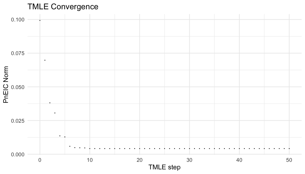
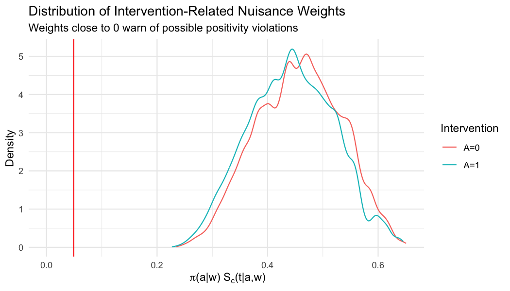
The component table is usually the most useful first view. plot(ConcreteEst, convergence = TRUE) shows the norm of the empirical EIC falling across update steps, and plot(ConcreteEst, gweights = TRUE) shows the distribution of the treatment/censoring nuisance weights with the positivity-risk threshold marked:

plot(ConcreteEst, convergence = TRUE)
plot(ConcreteEst, gweights = TRUE)

Key columns:

• PnEIC: empirical mean EIC for the component
• RelativeCriteria: original relative stopping threshold
• AbsoluteCriteria: absolute threshold supplied by EICStopAbsTol
• StopCriteria: threshold used by the selected rule
• ratio: abs(PnEIC) / StopCriteria
• check: whether that component passed the selected rule
• Converged: whether the overall update converged
• ConvergenceStep: update step where convergence was reached

Focus first on rows with check == FALSE, sorted by ratio.

components[check == FALSE][order(ratio, decreasing = TRUE)]

If there are failures, the output will identify which event/time/intervention combination is driving the problem:

Intervention	Time	Event	AbsPnEIC	StopCriteria	ratio	check
A=1	730	1	0.0048	0.0010	4.8	FALSE
A=0	730	1	0.0017	0.0010	1.7	FALSE

This pattern says the empirical EIC is still materially larger than the chosen threshold. Start with adaptive updating and a simpler learner library before loosening the stopping rule.

A worked rare-event example

The tables below are real getTmleDiagnostics() output from the PBC competing- risks example, targeting both death (event 1) and the rarer transplant (event 2) at four times. Under the relative rule, the rare event-2 components have a tiny standard-error scale, so their stopping threshold is minuscule and the ratio blows up even though the absolute PnEIC is small — the fit is flagged as not converged:

	Intervention	Time	Event	PnEIC	StopCriteria	ratio	check
6	A=1	730	2	-0.00145	0.00003	53.31646	FALSE
14	A=0	730	2	0.00057	0.00092	0.61972	TRUE
7	A=1	1460	2	-0.00083	0.00196	0.42503	TRUE
8	A=1	2190	2	0.00070	0.00248	0.28114	TRUE

Switching to the absolute rule (0.02 / sqrt(n)) judges those same small PnEIC values against a risk-scale tolerance. The spurious blow-up disappears — the worst ratio drops from roughly 50 to about 2 — leaving only a genuinely harder component that the escalation ladder addresses:

	Intervention	Time	Event	PnEIC	StopCriteria	ratio	check
7	A=1	1460	2	-0.00226	0.00113	1.99585	FALSE
8	A=1	2190	2	0.00220	0.00113	1.94196	FALSE
6	A=1	730	2	-0.00210	0.00113	1.85473	FALSE
14	A=0	730	2	0.00094	0.00113	0.83213	TRUE

This is the canonical rare-event pattern: under the relative rule a large ratio is driven by a near-zero threshold rather than by a meaningful targeting failure. The absolute rule removes that artifact; any remaining failures (here, the sparse transplant event) are real sparsity to work through with the escalation ladder below.

Recommended escalation ladder

Start simple and add flexibility only after the conservative analysis behaves as expected.

1. Run a conservative baseline

Use default Cox hazards and a small treatment Super Learner library.

Model <- list(
  arm = c("SL.mean", "SL.glm"),
  "0" = list(Censor = survival::Surv(time, event == 0) ~ arm + age + sex),
  "1" = list(Event = survival::Surv(time, event == 1) ~ arm + age + sex)
)

ConcreteArgs <- formatArguments(
  DataTable = trial,
  EventTime = "time",
  EventType = "event",
  Treatment = "arm",
  ID = "id",
  Intervention = makeITT(),
  TargetTime = c(365, 730),
  TargetEvent = 1,
  CVArg = list(V = 5),
  Model = Model,
  Verbose = FALSE
)

ConcreteEst <- doConcrete(ConcreteArgs)

2. Use adaptive updating

The adaptive method uses a line search with rollback and is the recommended first convergence fix. With EICStopRule = "relative" it accepts updates that reduce the target empirical EIC norm. With EICStopRule = "absolute" or "hybrid" it accepts updates that reduce the active component-wise stopping ratio.

ConcreteArgs$UpdateMethod <- "adaptive"
ConcreteArgs <- formatArguments(ConcreteArgs)
ConcreteEst <- doConcrete(ConcreteArgs)

3. Use an absolute risk-scale stopping rule for rare events

ConcreteArgs$UpdateMethod <- "adaptive"
ConcreteArgs$EICStopRule <- "absolute"
ConcreteArgs$EICStopAbsTol <- 0.02 / sqrt(nrow(ConcreteArgs$Data))
ConcreteArgs <- formatArguments(ConcreteArgs)
ConcreteEst <- doConcrete(ConcreteArgs)

Use this when the largest failing components have very small absolute PnEIC values but large ratios because the relative threshold is tiny. Treat it as a convergence sensitivity: report the stopping rule, compare estimates with the relative fit when available, and focus first on absolute risks and risk differences when event risks are very small.

A hybrid rule remains useful as a secondary sensitivity:

ConcreteArgs$UpdateMethod <- "adaptive"
ConcreteArgs$EICStopRule <- "hybrid"
ConcreteArgs$EICStopAbsTol <- 0.02 / sqrt(nrow(ConcreteArgs$Data))
ConcreteArgs <- formatArguments(ConcreteArgs)
ConcreteEst <- doConcrete(ConcreteArgs)

4. Increase iterations only if progress is continuing

ConcreteArgs$MaxUpdateIter <- 1000
ConcreteArgs <- formatArguments(ConcreteArgs)
ConcreteEst <- doConcrete(ConcreteArgs)

If the trace has flattened and the same tiny components remain, increasing iterations may not change the practical estimate.

5. Simplify or stabilize nuisance estimation

If abs(PnEIC) remains large, the issue may be nuisance instability rather than only the stopping threshold.

Try:

• simpler hazard learner libraries
• fewer high-variance learners for small trials
• stronger propensity-score truncation through MinNuisance
• fewer target times for initial debugging
• checking for arms with no events near the target time

Interpreting common patterns

Pattern	Likely meaning	Next step
Large ratio, tiny AbsPnEIC	Relative rule is too strict on a near-zero component	Try absolute with 0.02 / sqrt(n)
Large ratio, large AbsPnEIC	Targeting problem remains meaningful	Use adaptive update and inspect learners
Many failing components for censoring	Censoring or positivity instability	Check censoring by arm and covariates
Failure only for one rare event/time	Sparse target component	Report event counts and try absolute stopping
Norm decreases then rebounds	Update overshooting	Use UpdateMethod = "adaptive"

A reporting template

For trial reports or issue reports, record:

list(
  package_version = as.character(packageVersion("concrete")),
  update_method = ConcreteArgs$UpdateMethod,
  eic_stop_rule = ConcreteArgs$EICStopRule,
  eic_stop_abs_tol = ConcreteArgs$EICStopAbsTol,
  max_update_iter = ConcreteArgs$MaxUpdateIter,
  target_time = ConcreteArgs$TargetTime,
  target_event = ConcreteArgs$TargetEvent,
  event_counts = trial[, .N, by = .(arm, event)],
  components = getTmleDiagnostics(ConcreteEst, type = "components")
)

This is usually enough to understand whether a convergence issue is numerical, data-sparsity related, or learner related.